Waiting to Get Your Dissertation Accepted?
Last Updated on: 3rd February 2024, 01:40 am
A very useful technique in your toolkit of analyses for dissertations and theses, as well as real-world problems, is known as repeated measures. We choose this tool when we are measuring the same items, or people, multiple times. This could be over time, or under different circumstances—but the same participants.
In this article, I describe the two main tools—the paired t test and repeated measures ANOVA. I will focus on what you need to get the job done (among all the available info, tests, and outcomes).
What is Repeated Measures Analysis?
Many techniques are used to compare the means of two populations: for example, independent samples, t tests, and between-subjects ANOVA. These tools assume that the scores in different groups are independent of each other.
Sometimes, however, our objective is to analyze difference in means of populations that are related—when the attributes of the first population are not independent of the second (or third or many). Two situations involve data from related populations:
- We take repeated measurements from the same items or individuals at different points in time (repeated measures).
- We match the items or individuals according to some characteristic (matched samples).
In both cases, we are interested in the difference in measurements instead of the individual measurements. Taking repeated measurements on the same items or individuals assumes that they will behave similarly if treated alike. Our objective is to demonstrate that any differences between two measurements of the same individuals are explained by a treatment.

An Example?
Let’s say we are evaluating the effectiveness of a training program for a group of management candidates. We administer a test of knowledge to the same participants, using several different training methods. We’re trying to determine if there is any difference (hopefully, improvement) in knowledge as a result of the training, and to see if the effectiveness is influenced by the type of training. This is a repeated measures analysis.
Or, we might be interested in the improvement in skill level among technicians over time, as they gain experience in a task (like assembling electronic parts). We test them at points in time to see if there is a time-related improvement—a learning curve.
In both instances, measurements can be made at multiple times (after different training events; or at different points in time).
Get Your Dissertation Accepted On Your Next Submission

Paired t Test
One technique for this task is the paired t test for the mean difference in related populations. The paired t test is used when there are only two measures of the same participants.
For each participant, we collect pre- and post-treatment scores, compute the difference (xD = x2 – x1), then compute the average difference (xD) for the sample of participants (the sum of the differences, xD, divided by the sample size, n).
The null hypothesis for a paired t test is that there is no difference in the means of two related populations:
H0: μD = 0 (where μD = the average difference in scores for the population)
against the alternative that the means are not the same:
H1: μD ≠ 0.
As in all hypothesis tests, we compute a test statistic:

(where μD = hypothesized mean difference, and SD = sample standard deviation of differences)
As usual, we test the hypothesis with the tSTAT using its p value compared to the level of significance, α.
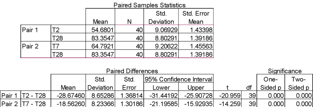
Following our example of 40 management trainees, here are the outputs from SPSS for a paired samples test. We actually performed two statistical tests, one between training days 2 and 28; and one between training days 7 and 28. In both cases, we reject the null because the p value is less than α = .05. We conclude that the mean difference in scores between two points in time is statistically significant (increasing by 28.7 points from day 2 to day 28).
Repeated Measures ANOVA
We use the paired samples t test to evaluate whether means differ across collections under two different treatments; or between scores obtained at two different points in time. If there are more than two treatments or times, we use a one-way repeated measures ANOVA; also called within-subjects ANOVA.
Hypotheses
For a problem with three measurements of the same participants (points in time or conditions), here are the hypotheses:
H0: μ1 = μ2 = μ3 (where μi = the average score for measurement i);
meaning, the population mean scores (measurements) for persons (items) assessed at these three points (conditions) are equal;
against the alternative that the means are not the same:
We test the differences using samples of scores at each measurement point. There is no limit to the number of measurements that can be compared using repeated measures ANOVA;
Setting up in SPSS
This test is easily set up in SPSS. To start, select
Analyze > General Linear Model > Repeated Measures.
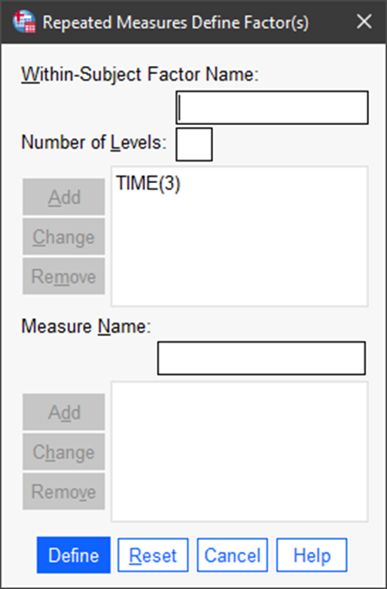
Then, provide the within-subject factor name and number of levels and Add as shown in the figure. In this example, the factor that we are evaluating is TIME. It has three levels: T2, T7, and T28. These represent the points in time at which we are conducting the test of the trainees, so we can determine if their knowledge or skill is changing (improving) over time.
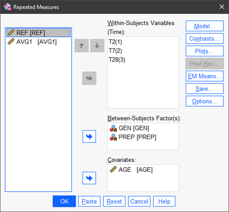
The next step is to define the analysis. The within-subject factor, TIME, is already populated. In this next screen we can add between-subject factors (categorical variables) that are potential influences on test scores (in our example). And, we can add a numerical covariate that is also postulated to influence the response.
Note in the next figure that we have added gender (GEN), whether or not the trainee had a prep course (PREP), and age (AGE).
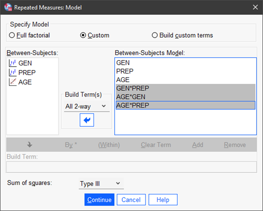
Then, we can set up the analysis by selecting Model. Here, we can add the three between-subject factors and three two-factor interactions. Then click on Continue.
We can then set up some graphs of the two-factor interactions, which provides additional evidence of their influence on the response variable, test scores.
Under Save we direct SPSS to save the unstandardized residuals. These are the model error terms They represent the difference between predicted and actual values of the response variable, for evaluation of the ANOVA assumptions. They are saved in the SPSS data file.
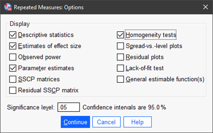
Under Options we tell SPSS which outputs we need to evaluate the predictive model and the influence of the various predictors.
Executing Repeated Measures ANOVA
After the problem is set up in SPSS, we can simply click on OK in the main screen.
Test for Sphericity
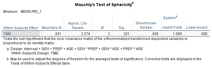
We first test for sphericity. Sphericity refers to the condition where the variances of the differences between all combinations of related groups are equal. If this assumption is violated, the F statistic becomes inflated and the results of the repeated measures ANOVA become unreliable. Mauchly’s test of sphericity is used to test whether or not the assumption of sphericity is met in a repeated measures ANOVA.
The null hypothesis is
H0: the variances of the group differences are equal (sphericity).
In the SPSS output, if the p value (Sig.) < level of significance (α =.05 for this example), reject the null and conclude that the assumption of sphericity is violated. If p > α, then fail to reject the null and conclude that the assumption of sphericity holds. In our example, Mauchly’s W = .931, and its p value = .321. We conclude that the assumption is not violated.
When the assumption is violated, the risk of a Type I error (false positive—detecting an effect that does not in fact exist) is higher than reported. There are two remedies for this situation: use downwardly adjusted df values or use MANOVA instead of repeated measures ANOVA (see Warner, 2013).
Test Repeated Measures Hypotheses
Now, we test the repeated measures hypotheses. With sphericity assumed (now that we tested for it), we use the first line of the Tests of Within-Subjects Effects table to test the hypothesis (equal population means for test scores at each point in time). We use the F test and its associated p value (Sig.).
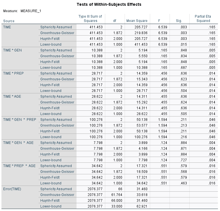
In our example, F = 6.539, p = .003 < .05. We reject the null hypothesis and conclude there is a difference in mean scores at the three points in time.
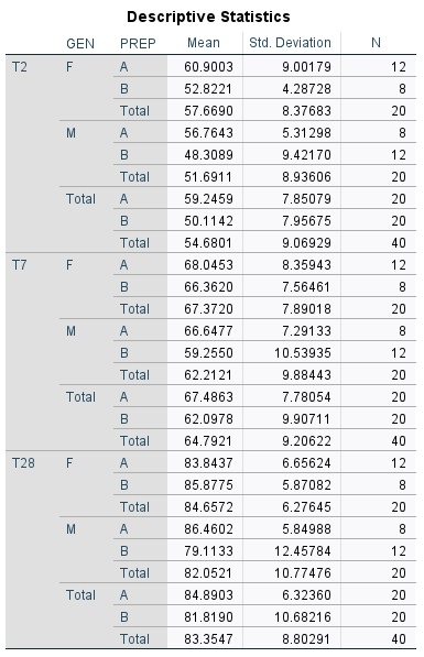
We now refer to the Descriptive Statistics table, which shows that the mean scores for each of the time points (T2, T7, and T28) are 54.7, 64.8, and 83.4 respectively. But, wait! There’s more.
Interpreting Results of Repeated Measures
We still have three issues to address:
- What about the between-subjects factors and covariate?
- What about the final predictive model of our test scores? Which factors/covariates are significant predictors?
- Is there any significant interaction between factors/covariates?
Model-Building
Let’s start with issue #2. We would not have a thorough, complete analysis if we stopped here. A one-time run of ANOVA with predictors is incomplete. Instead, we need to find the best predictive model of the dependent variable, through model-building. I explain this in detail in three other articles on multiple linear regression, ANOVA, and two-factor interactions.
The point is, in ANOVA as in regression, we simply cannot make a truthful statement about the influence of any single factor without simultaneously considering all influential factors. These are expressed in a final mathematical model, developed through a rigorous, sequential model-building process.
Recall that in our example, we began with one within-subjects factor (TIME), two between-subjects factors (GEN and PREP), and a covariate (AGE). We found TIME to be a significant factor. But, when we look at the Tests of Between-Subjects Effects table, we see that not all of the factors and interactions are significant (based on p [Sig.] < .05). So, we are not yet ready to address either issue #1 or issue #3.
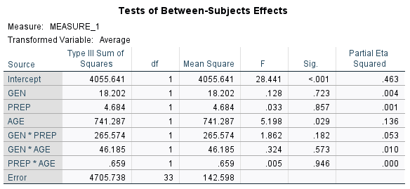
We run through a series of purposeful model runs, trying different combinations, seeing which remain significant and which are clearly not. We pay attention to p values for each term and Partial Eta Squared (η2). Partial η2 ranges from 0 to 1, and measures the proportion of variance in the response variable explained by each factor while accounting for variance explained by other factors in the model. It is a measure of the influence of each CF, and can be useful in variable selection.
After the model-building process, we have addressed issue #2 and can address issue #1. In our example, we have a final model consisting of the TIME variable plus a between-subjects factor (PREP), the covariate (AGE), and the interaction (GEN*PREP). These we consider the significant predictors of test scores for the example.
The Tests of Between-Subjects Effects table for the final model looks like this:
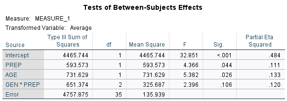
Note that we have two of the factors with p values less than .05. The factor interaction has a p value of .106. I have written in other articles about using a liberal variable selection criterion to avoid missing variable bias and to build the best predictive model.
So, in this case, with a factor interaction that is marginally significant, I turn to the graph of estimated marginal means to see if an interaction is indicated. I also know that the sample size in this example was relatively low (n = 40). So, for the purposes of this analysis, I include the factor interaction in the final model.
Factor Interactions
A factor interaction exists when the influence of one factor on the response variable depends on the value of another factor. In our final model of test scores, we have one significant factor interaction: GEN*PREP. Interactions provide some interesting insights, and this example is no different. We interpret factor interactions best with graphs.
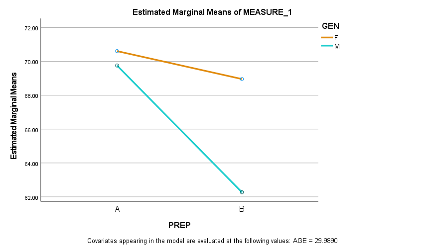
Here we can see that the between-subjects factor, GEN, is a moderator of the relationship between PREP and test scores. GEN, by itself, is not a statistically significance predictor, but it is a significant influence on the PREP vs. test score relationship.
A value of “A” for PREP is a “yes”—the individual had the prep course. So, not surprisingly, for all trainees, average test scores (over three measurements) are higher with the prep course. But, what is not obvious until we examine the graph is that the prep course appears to be more effective for males than for females. Test scores without the prep course are lower for males than for females, but are fairly close with the prep course.

Factor interactions often provide some of the most interesting insights in any multivariate analysis.
Predictive Model in Repeated Measures
We tested the hypotheses, and concluded that time, the prep course, and age are statistically significant predictors of test scores. But, there are questions remaining. One is, how sensitive are scores to the predictors? There are useful tables provided by SPSS, including Descriptive Statistics and Estimated Marginal Means. But, the table most useful for the predictive model is the Parameter Estimates table:
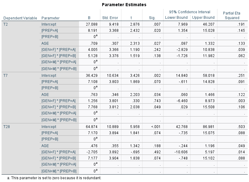
This table shows the effects from each value or level of the predictors. To predict a value for test scores, we apply estimates of the specific effects, as in this example:
Grand mean of test scores at day 28 = 64.874
Prep course = A (“yes”) = 1 × 7.170 = 7.170
Age (28) = 28 × 0.476 = 13.328
Female trainee (GEN = F)
Interaction GEN*PREP (F, A) = 1 × (-2.705) = -2.705
Predicted score at day 28 = 82.667.
Final thoughts
In dissertations, theses, and real-world analyses, we use various multivariate tools to evaluate the influence of multiple factors on measurable phenomena. When we are measuring the phenomenon multiple times for the same individuals or items, the best tool is a repeated measures analysis—either a paired t test or a repeated measures ANOVA.
The beauty of repeated measures ANOVA is that we can assess the influence of time or multiple conditions; while at the same time evaluating the influence of other factors and covariates.
The result is an understanding of the sensitivity of the phenomenon to factors and influences. And, we have the capability to predict its behavior or performance as a function of time, or multiple measurements, or other factors using a predictive mathematical model.
References
- IBM Corporation. (2022). IBM SPSS Statistics for Windows, Version 28.0. IBM Corp.
- Levine, D. M., Berenson, M. L., Krehbiel, T. C., & Stephan, D. F. (2011). Statistics for managers using MS Excel. Prentice Hall/Pearson.
- Statology. (2022). Sphericity. https://www.statology.org/mauchlys-test-of-sphericity
- Warner, R. M. (2013). Applied statistics: From bivariate through multivariate techniques. Sage.